RF: Noise to Power Ratio (NPR) Test

Introduction
NPR, or Noise to Power Ratio, is a figure of merit describing an amplifier's linearity.  When I say linearity, I am referring to the amplifier's ability to keep it's gain flat versus output power.  Of course it's deeper than this but this is a good way to understand it.

Now many people know of different types of linearity figures of merit, OIP3 for instance.  Unfortunately, OIP3 is only good for certain instances, single carriers or very few carriers.  But what about OFDM or QAM modulation techniques that have closely spaced signals?

This is where an NPR test is useful.  It takes into account a lot of different carriers during the test and tests how linear the amplifier is.  I'm not going into great detail of the mathematics but I will indicate the basics of how it works

The Basics
The most common way to perform an NPR test is to use 5 main devices in the lab:

1. AWGN source (Noise Source): This is used to simulate the many frequency tones.
2. Bandpass Filter: A filter used to bandlimit the noise into a usable bandwidth. Generally, this is the waveform's bandwidth.
3. Notch Filter: A filter, or method, of taking out a small section of the noise, creating a "notch" in the middle of the waveform.
4. AUT: This is the amplifier that is being tested, generally a power amplifier.
5. Spectrum Analyzer: Used to take the measurements. (Could be a Network Analyzer)

So in order to perform the test, you need to hook up the source to the bandpass filter then the notch filter.  Followed by this is the AUT and finally the Spectrum Analyzer.  Generally the notch will be the bandwidth of the signal separation.

Ultimately, the point of this setup is to see how much the notch is filled after the sample noise waveform passes through the amplifier.  This idea is based on intermod theory.  When many tones are very close together they will "intermodulate" with each other and form harmonics at other close frequencies.  This is how the notch "fills up," by the intermodulation harmonics from other tones.  Based on this we can find how linear the amplifier is relative to different noise power levels.

Conclusion

So there is a lot here that wasn't said but I hope you have a basic idea on what the purpose and why NPR works.  An NPR test is basically using intermod theory on a large number of tones to see how much they modulate with each other.  After that, it's simple math using dBc/Hz reference powers of Spectral Density.  If you desire more information or examples, I'll be more than happy to help.  Just email me or comment. Later!

-------------------------------

Justin Coulston

justin.coulston@gmail.com

RF: Broadband Matching

Introduction
Today at work, I came to the conclusion that Broadband matching is a fine art.  It takes years of experience to understand and get it right.  Even the most experienced RF Engineers still have issues developing a matching network for amplifiers and power transistors.

I'm going to give a brief overview of Broadband matching and how it applies to the RF engineer.

The Basics
A matching network is simply any network that can transform impedances from it's input to output.  Generally, they consist of either LC networks or microstrip equivalents.  They come in the form of filter type matches.  I have mostly used strings of networks with the high pass and low pass structure.

There are many ways to match networks and many structures you can use.  At low frequencies (under 1 GHz) and at narrow bandwidths (under 100 MHz) it's generally easier to match using the Smith Chart.  At higher frequencies and higher bandwidths, I recommend a more trial and error approach.  This is what broadband matching entails (higher bandwidths).  There is no single method to broadband matching, so I'll show you my method and then only with amplifier/transistors.

My Method
So let's say we have an RF amplifier that is denoted like so:

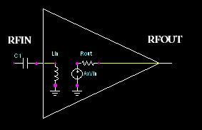
Every amp has an inherent input impedance and output impedance.  This is modeled by something like so:

Now generally, input impedances are meant to be extremely high (Megaohms in Op-Amps) but in RF amps they can be very small (sometimes 2 - 3 ohms).  The output can be almost anything, but generally smaller.

Now something to notice, is the inherent resistances.  Most of the time they are not strictly resistive and will be reactive as well.  I noticed today that the amp I was using was in fact inductive at high frequencies.  So I had to match accordingly.  

Since Rin = Lin, I began my matching with a series capacitor like so:

So you see, I used the internal inductor as my first component, then use the series capacitor to complete this first part of the match (High Pass Filter).

To shorten this post up a little bit, I will say that you will then put a shunt capacitor as the next component, then a series inductor, etc, etc.  Repeat those until you have a match.  Do the same for the output.

Now the big question you'll be asking is "what about the values?"  Well this is where the art comes in.  It's not a very simple topic to go through.  This is completely dependent on what frequency return loss goals you have and how many networks you have. I generally use an optimizer in Agilent's ADS Simulation Software (EESof).

But I will give you a general overview of what "type" of values you'll need for certain frequency ranges:

HIGH FREQUENCY (500MHz-2GHz)

• Shunt C: Very low values (0.1pF - 2pF)
• Shunt L: Medium values (50nH - 100nH)
• Series C: Medium RF values (20pF - 50pF) [These are more dependent on other factors]
• Series L: Very low values (1.6nH - 15nH)

LOW FREQUENCY ( < 500MHz)

• Shunt C: Medium values (100pF - 1uF)
• Shunt L: High Values (1uH - 100uH) [This is a guesstimate]
• Series C: High RF values (1000pF - 10uF)
• Series L: Medium values (100nH - 10uH)

I hope this post is somewhat useful.  I know it's vague on details but I want to give you an idea on broadband matching.  I can't really write a whitepaper on it for a post.  If you have specific questions email/comment and ask.  Later

--------------------

Justin Coulston

justin.coulston@gmail.com

Component Selection: Amplifier Nonlinearity

Introduction

A linear device is any device that changes due to a linear relationship between it's input and output.  For example, a 3dB attenuator will always attenuate 3dB of power regardless of power (Of course this doesn't take into account the breakdown voltage of components).  Another example is amplifiers in small-signal applications.  In small signal applications the output voltage of an amplifier can be modeled by the following equation:

where R0 and R1 are DC Voltage and Voltage Gain of an amplifier.  This is typical usage of amplifiers.  Unfortunately, Amplifiers won't continue to amplify signals infinitely.  This is why with large-signals amplifiers have "non-linear" behavior...

The Non-Linear Amplifier

So what causes these non-linearities? Non-linearity occurs due to device saturation, or the point where the device can no longer provide any more power.  In the below graph, you can see an amplifier's input power to output power characteristics.  For smaller input power signals, the line is very straight, or linear.  As the input power draws near to 0 dBm, you can see it starts to roll off.  This indicates that the gain is no longer the same and is in fact dropping as the input power rises.

From Maxim-IC.Com

If the input power continues to rise, eventually you would see a straight horizontal line indicating it has hit saturation.  This output power level is known as the Saturation Level of the amplifier (simple enough).

Many non-linear amps can be modeled using a Taylor Expansion style equation:

This is the equation where you can derive the second, third, fourth, etc harmonics.  If you were to input a cos(wt) into the equation you would see components of many frequencies (I'll do this math at a later date).  This is also where the non-linear figure of merit, 3rd Order Intercept Point (IP3), comes from.  If you have a signal Vin = cos(w0t) + cos(w1t) into the equation you would see where the third-order harmonic comes into play.  Very interesting math to go through (again...at a later date)

Summary

Granted, this is a very basic explanation of non-linear behavior but it's important to know where it comes from when working with power amplifiers especially.  I put this under Component Selection mainly because of the importance this idea is when picking out amplifiers.  Be sure that your amplifier is as linear as possible when selecting an amp, otherwise many unexpected problems can arise.  If you have specific questions feel free to ask. Enjoy!

------------------------

Justin Coulston

justin.coulston@gmail.com

In Practice: Quick and On-Time Engineering

So I've come to realize today how serious, and easy, it is to miss something when you're designing hardware.  It's amazing how easy it is to miss that small tid-bit of information that normally you wouldn't have to worry about.

For instance, when working with amplifiers in High Frequency applications you have to worry about a lot: Output 3rd Order Intercept (OIP3), 1-dB Compression (P1dB), Gain Flatness, Power Saturation Point, Noise Figure (NF), Input and Output Impedance, etc.

This type of information is all critical when designing a system at high frequencies.  But if you miss one, issues will arise.  For instance, if you don't measure P1dB for your amplifier, you may expect gain to continue for any input power, but once you put the amp in the circuit, you may realize that you don't get the power expected.  If you have a P1dB of 15 dBm and a gain of 10 dB, when you put 10 dBm into the amp, there is a VERY HIGH possibility you won't get 25dBm out, and if you do you'll have plenty of distortion.

So the point of this is to say that it's very important to take your time when engineering.  When setting out to design something, first you need to know where you are going.  I have found this to be the best piece of advice I can give someone in engineering.

How can you go anywhere without the direction.  So learn the direction first.  Then find out what will take you there with metrics.  Know how much power you'll need before hand.  Know how big your circuit can be.  Know everything to make it work before you start, with metrics.

Finally, layout what information you'll need to realize these metrics.  Not all metrics are directly measurable.  So you must find out how to measure it.  For instance, amplifier linearity is not directly measurable.  One way to characterize this is to use an OIP3 measurement.  The common way is to add two signals 1 MHz apart and measure the intermods.

This is what you have to figure out.  So to summarize:

1. Know where you're going.  Know your goal
2. Determine your metric requirements whether measurable or not.
3. Figure out how to measure the objective and subjective metrics and then measure them for your proposed design

That's it.  It's simple and I could go in more detail but this is supposed to be the basics...

--------------------

Justin Coulston

justin.coulston@gmail.com